Introduction: Listen up, cluster admins. If you rely on networked storage, drop what you are doing right now because a critical Kubernetes CSI Driver for NFS flaw just hit the wire, and it is an absolute nightmare.
I’ve spent 30 years in the trenches of tech infrastructure, and I know a disaster when I see one.
This vulnerability isn’t just a minor glitch; it actively allows attackers to modify or completely delete your underlying server data.

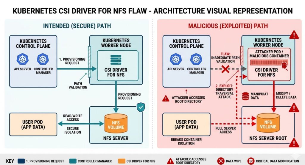
Table of Contents
Why This Kubernetes CSI Driver for NFS Flaw Matters
Back in the early days of networked file systems, we used to joke that NFS stood for “No File Security.”
Decades later, the joke is on us. This new Kubernetes CSI Driver for NFS flaw proves that legacy protocols wrapped in modern containers still carry massive risks.
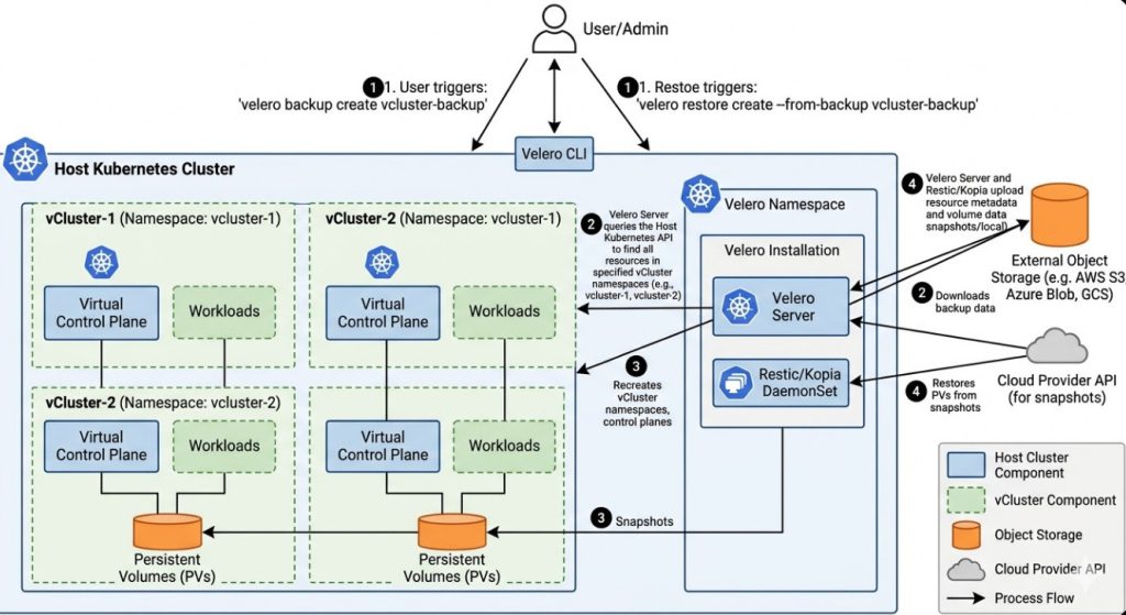
So, why does this matter? Because your persistent volumes are the lifeblood of your applications.
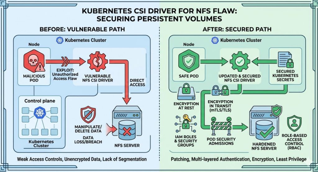
If an attacker exploits this Kubernetes CSI Driver for NFS flaw, they bypass container isolation entirely.
They gain direct, unfettered access to the NFS share acting as your storage backend.
That means your databases, customer records, and application states are sitting ducks.
The Anatomy of the Exploit
Let’s get technical for a minute. How exactly does this happen?
The Container Storage Interface (CSI) is designed to abstract storage provisioning. It’s supposed to be secure by design.
However, this specific Kubernetes CSI Driver for NFS flaw stems from inadequate path validation and permission boundaries within the driver itself.
When a malicious actor provisions a volume or manipulates a pod’s spec, they can perform a directory traversal attack.
This breaks them out of their designated sub-directory on the NFS server.
Suddenly, they are at the root of the share. From there, it’s game over.
Immediate Remediation for the Kubernetes CSI Driver for NFS Flaw
You do not have the luxury of waiting for the next maintenance window.
You need to patch this Kubernetes CSI Driver for NFS flaw immediately to protect your infrastructure.
For the complete, unvarnished details, check the official vulnerability documentation.
First, audit your clusters to see if you are running the vulnerable driver versions.
# Check your installed CSI drivers
kubectl get csidrivers
# Look for nfs.csi.k8s.io and check the deployed pod versions
kubectl get pods -n kube-system -l app=nfs-csi-node -o=jsonpath='{range .items[*]}{.spec.containers[*].image}{"\n"}{end}'
If you see a vulnerable tag, you must upgrade your Helm charts or manifests right now.
Step-by-Step Patching Guide
Upgrading is usually straightforward, but don’t blindly run commands in production without a backup.
Here is my battle-tested approach to locking down this Kubernetes CSI Driver for NFS flaw.
- Snapshot Everything: Take a storage-level snapshot of your NFS server. Do not skip this.
- Update the Repo: Ensure your Helm repository is up to date with the latest patches.
- Apply the Upgrade: Roll out the patched driver version to your control plane and worker nodes.
- Verify the Rollout: Confirm all CSI pods have restarted and are running the safe image.
You can also refer to our guide on [Internal Link: Kubernetes Role-Based Access Control Best Practices] to limit blast radius.
Long-Term Strategy: Moving Beyond NFS?
This Kubernetes CSI Driver for NFS flaw should be a massive wake-up call for your architecture team.
NFS is fantastic for legacy environments, but it relies heavily on network-level trust.
In a multi-tenant Kubernetes cluster, network-level trust is a dangerous illusion.
You might want to consider block storage (like AWS EBS or Ceph) or object storage (like S3) for critical workloads.
These modern storage backends integrate more cleanly with Kubernetes’ native security primitives.
They enforce strict IAM roles rather than relying on IP whitelisting and UID matching.

How to Audit for Historical Breaches
Patching the Kubernetes CSI Driver for NFS flaw stops future attacks, but what if they are already inside?
You need to comb through your NFS server logs immediately.
Look for anomalous file deletions, modifications to ownership (chown), or unexpected directory traversals (../).
If your audit logs are disabled, you are flying blind.
Turn on robust auditing at the NFS server level today. It is your only real source of truth.
# Example of enforcing security contexts to limit NFS risks
apiVersion: v1
kind: Pod
metadata:
  name: secure-nfs-client
spec:
  securityContext:
    runAsNonRoot: true
    runAsUser: 1000
    fsGroup: 2000
  containers:
  - name: my-app
    image: my-app:latest
Reviewing Your Pod Security Standards
Are you still allowing containers to run as root?
If you are, you are handing attackers the keys to the kingdom when a flaw like this drops.
Enforce strict Pod Security Admissions (PSA) to ensure no pod can mount arbitrary host paths or run as root.
This defense-in-depth strategy is what separates the pros from the amateurs.
Frequently Asked Questions (FAQ)
- What is the Kubernetes CSI Driver for NFS flaw? It is a severe vulnerability allowing attackers to bypass directory restrictions and modify or delete data on the underlying NFS server.
- Does this affect all versions of Kubernetes? The flaw resides in the CSI driver itself, not the core Kubernetes control plane, but it affects any cluster utilizing the vulnerable driver versions.
- Can I just use read-only mounts? Read-only mounts mitigate data deletion, but if the underlying NFS server is exposed, path traversal could still lead to sensitive data exposure.
- How quickly do I need to patch? Immediately. Active exploits targeting infrastructure vulnerabilities are weaponized within hours of disclosure.
- Is AWS EFS affected? Check the specific driver you are using. If you use the generic open-source NFS driver, you are likely vulnerable. Cloud-specific drivers (like the AWS EFS CSI driver) have their own release cycles and architectures.
Conclusion: The tech landscape is unforgiving. A single Kubernetes CSI Driver for NFS flaw can undo months of hard work and destroy your data integrity. Patch your clusters, audit your logs, and stop trusting legacy protocols in modern, multi-tenant environments. Do the work today, so you aren’t writing an incident report tomorrow. Thank you for reading the DevopsRoles page!