Introduction: I am completely sick and tired of modern web browsing, and if you are looking to deploy Pi-Hole with Docker, you are exactly in the right place.
The internet used to be clean, fast, and text-driven.
Today? It is an absolute swamp of auto-playing videos, invisible trackers, and malicious banner ads.

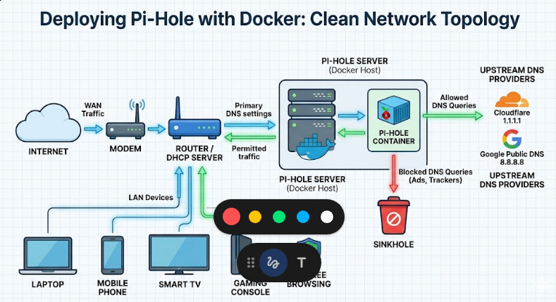
Table of Contents
- 1 The Madness Ends When You Deploy Pi-Hole with Docker
- 2 Why Containerization is the Only Way
- 3 Prerequisites to Deploy Pi-Hole with Docker
- 4 Step 1: The Configuration to Deploy Pi-Hole with Docker
- 5 Step 2: Firing Up the Container
- 6 Step 3: Forcing LAN Traffic Through the Sinkhole
- 7 Dealing with Ubuntu Port 53 Conflicts
The Madness Ends When You Deploy Pi-Hole with Docker
Ads are literally choking our bandwidth and ruining user experience.
You could install a browser extension on every single device you own, but that is a rookie move.
What about your smart TV? What about your mobile phone apps? What about your IoT fridge?
Browser extensions cannot save those devices from pinging tracker servers 24/7.
This is exactly why you need to intercept the traffic at the network level.
DNS Blackholing Explained
Let’s talk about DNS. The Domain Name System.
It’s the phonebook of the internet. It translates “google.com” into a server IP address.
When a website tries to load a banner ad, it asks the DNS for the ad server’s IP.
A standard DNS says, “Here you go!” and the garbage ad immediately loads on your screen.
Pi-Hole acts as a rogue DNS server on your local area network (LAN).
When an ad server is requested, Pi-Hole simply lies to the requesting device.
It sends the request into a black hole. The ad never even downloads.
This saves massive amounts of bandwidth and instantly speeds up your entire house.
Why Containerization is the Only Way
So, why not just run it directly on a Raspberry Pi OS bare metal?
Because bare-metal installations are messy. They conflict with other software.
When you deploy Pi-Hole with Docker, you isolate the entire environment perfectly.
If it breaks, you nuke the container and spin it back up in seconds.
I’ve spent countless nights fixing broken Linux dependencies. Docker ends that misery forever.
It is the industry standard for a reason. Do it once, do it right.
Prerequisites to Deploy Pi-Hole with Docker
Before we get our hands dirty in the terminal, we need the right tools.
You cannot build a reliable server without a solid foundation.
First, you need a machine running 24/7 on your home network.
A Raspberry Pi is perfect. An old laptop works. A dedicated NAS is even better.
I personally use a cheap micro-PC I bought off eBay for fifty bucks.
Next, you must have the container engine installed on that specific machine.
If you haven’t installed it yet, stop right here and fix that.
Read the official installation documentation to get that sorted immediately.
You will also need Docker Compose, which makes managing these services a breeze.
Finally, you need a static IP address for your server machine.
If your DNS server changes its IP, your entire network will lose internet access instantly.
I learned that the hard way during a Zoom call with a major enterprise client.
Never again. Set a static IP in your router’s DHCP settings right now.
Step 1: The Configuration to Deploy Pi-Hole with Docker
Now for the fun part. The actual code.
I despise running long, messy terminal commands that I can’t easily reproduce.
Docker Compose allows us to define our entire server in one simple, elegant YAML file.
Create a new folder on your server. Let’s simply call it pihole.
Inside that folder, create a file explicitly named docker-compose.yml.
Open it in your favorite text editor. I prefer Nano for quick SSH server edits.
For more details, check the official documentation.
version: "3"

# Essential configuration to deploy Pi-Hole with Docker
services:
  pihole:
    container_name: pihole
    image: pihole/pihole:latest
    ports:
      - "53:53/tcp"
      - "53:53/udp"
      - "67:67/udp"
      - "80:80/tcp"
    environment:
      TZ: 'America/New_York'
      WEBPASSWORD: 'change_this_immediately'
    volumes:
      - './etc-pihole:/etc/pihole'
      - './etc-dnsmasq.d:/etc/dnsmasq.d'
    restart: unless-stopped
Breaking Down the YAML File
Let’s aggressively dissect what we just built here.
The image tag pulls the absolute latest version directly from the developers.
The ports section is critical. Port 53 is the universal standard for DNS traffic.
If port 53 isn’t cleanly mapped, your ad-blocker is completely useless.
Port 80 gives us access to the beautiful web administration interface.
The environment variables set your server timezone and the admin dashboard password.
Please, for the love of all things tech, change the default password in that file.
The volumes section ensures your data persists across reboots.
If you don’t map volumes, you will lose all your settings when the container updates.
I once lost a custom blocklist of 2 million domains because I forgot to map my volumes.
It took me three furious days to rebuild it. Learn from my pain.
Step 2: Firing Up the Container
We have our blueprint. Now we finally build.
Open your terminal. Navigate to the folder containing your new YAML file.
Execute the following command to bring the stack online:
docker-compose up -d
The -d flag is crucial. It stands for “detached mode”.
This means the process runs in the background silently.
You can safely close your SSH session without accidentally killing the server.
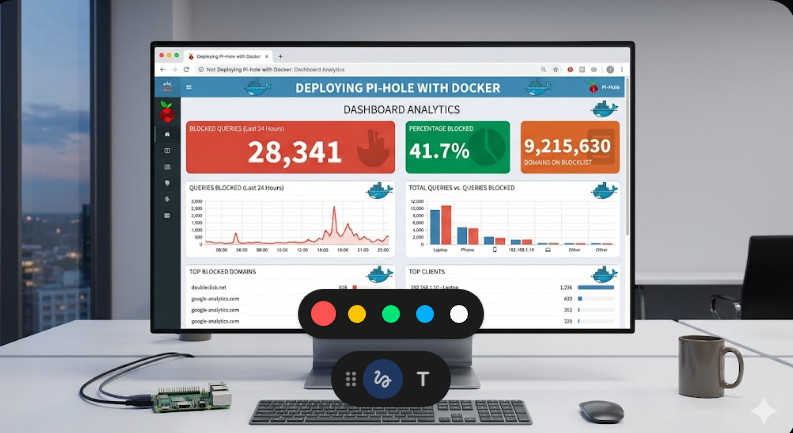
Within 60 seconds, your ad-blocking DNS server will be fully alive.
To verify it is running cleanly, simply type docker ps in your terminal.
If you ever need to read the raw source code, check out their GitHub repository.
You should also heavily consider reading our other guide: [Internal Link: Securing Your Home Lab Network].
Step 3: Forcing LAN Traffic Through the Sinkhole
This is where the magic actually happens.
Right now, your server is running, but absolutely no one is talking to it.
We need to force all LAN traffic to ask your new server for directions.
Log into your home ISP router’s administration panel.
This is usually located at an address like 192.168.1.1 or 10.0.0.1.
Navigate deeply into the LAN or DHCP settings page.
Find the configuration box labeled “Primary DNS Server”.
Replace whatever is currently there with the static IP of your container server.
Save the settings and hard reboot your router to force a DHCP lease renewal.
When your devices reconnect, they will securely receive the new DNS instructions.
Boom. You just managed to deploy Pi-Hole with Docker across your whole house.
Dealing with Ubuntu Port 53 Conflicts
Let’s talk about the massive elephant in the room: Port 53 conflicts.
When you attempt to deploy Pi-Hole with Docker on Ubuntu, you might hit a wall.
Ubuntu comes with a service called systemd-resolved enabled by default.
This built-in service aggressively hogs port 53, refusing to let go.
If you try to run your compose file, the engine will throw a fatal error.
It will loudly complain: “bind: address already in use”.
I see this panic question on Reddit forums at least ten times a day.
To fix it, you need to permanently neuter the systemd-resolved stub listener.
sudo nano /etc/systemd/resolved.conf
Uncomment the DNSStubListener line and explicitly change it to no.
Restart the system service, and now your container can finally bind to the port.
It is a minor annoyance, but knowing how to fix it separates the pros from the amateurs.

FAQ Section
- Will this slow down my gaming or streaming? No. It actually speeds up your network by preventing your devices from downloading heavy, malicious ads. DNS resolution takes mere milliseconds.
- Can I securely use this with a VPN? Yes. You can set your VPN clients to use your local IP for DNS, provided they are correctly bridged on the same virtual network.
- What happens if the server hardware crashes? If the machine stops, your network loses DNS. This means no internet. That’s exactly why we use the robust
restart: unless-stoppedrule! - Is it legal to deploy Pi-Hole with Docker to block ads? Absolutely. You completely control the traffic entering your own private network. You are simply refusing to resolve specific tracker domain names.
Conclusion: Taking absolute control of your home network is no longer optional in this digital age. It is a strict necessity. By choosing to deploy Pi-Hole with Docker, you have effectively built an impenetrable digital moat around your household. You’ve stripped out the aggressive tracking, drastically accelerated your page load times, and completely reclaimed your privacy. I’ve run this exact, battle-tested setup for years without a single catastrophic hiccup. Maintain your community blocklists, keep your underlying container updated, and enjoy the clean, ad-free web the way it was originally intended. Welcome to the resistance. Thank you for reading the DevopsRoles page!